Posterior distributions and sampling

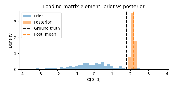
This example shows how the posterior distribution learned by GFA concentrates around ground truth parameter values, in contrast to the diffuse prior distribution before seeing data.

Imports

import logging

import matplotlib.pyplot as plt
import numpy as np

from latents.callbacks import LoggingCallback
from latents.gfa import GFAFitConfig, GFAModel
from latents.gfa.config import GFASimConfig
from latents.gfa.simulation import simulate
from latents.observation import (
    ObsParamsHyperPrior,
    ObsParamsHyperPriorStructured,
    ObsParamsPrior,
)

logging.basicConfig(level=logging.INFO, format="%(message)s")

Setup: simulate and fit

We simulate data with known ground truth and fit a GFA model. See Fitting GFA to simulated data for details.

n_samples = 100
y_dims = np.array([10, 10, 10])
x_dim = 7

sparsity_pattern = np.array(
    [
        [1, 1, 1, np.inf, 1, np.inf, np.inf],
        [1, 1, np.inf, 1, np.inf, 1, np.inf],
        [1, np.inf, 1, 1, np.inf, np.inf, 1],
    ],
)

MAG = 100
hyperprior = ObsParamsHyperPriorStructured(
    a_alpha=MAG * sparsity_pattern,
    b_alpha=MAG * np.ones_like(sparsity_pattern),
    a_phi=1.0,
    b_phi=1.0,
    beta_d=1.0,
)

sim_config = GFASimConfig(
    n_samples=n_samples,
    y_dims=y_dims,
    x_dim=x_dim,
    snr=1.0,
    random_seed=0,
)

sim_result = simulate(sim_config, hyperprior)
Y = sim_result.observations
obs_params_true = sim_result.obs_params

# Fit the model
config = GFAFitConfig(
    x_dim_init=10,
    fit_tol=1e-8,
    max_iter=20000,
    random_seed=0,
    prune_x=True,
    prune_tol=1e-7,
    save_c_cov=True,  # Required for posterior sampling
)

model = GFAModel(config=config)
model.fit(Y, callbacks=[LoggingCallback()])

GFAModel(fitted=True, config=GFAFitConfig(x_dim_init=10, fit_tol=1e-08, max_iter=20000, prune_x=True, prune_tol=1e-07, save_x=False, save_c_cov=True, save_fit_progress=True, random_seed=0, min_var_frac=0.001))

Access prior and posterior

GFAModel provides unified access to both the prior and posterior via model.obs_prior and model.obs_posterior.

print(f"Prior:     {model.obs_prior}")
print(f"Posterior: {model.obs_posterior}")

Prior:     ObsParamsPrior(hyperprior=ObsParamsHyperPrior(a_alpha=1e-12, b_alpha=1e-12, a_phi=1e-12, b_phi=1e-12, beta_d=1e-12))
Posterior: ObsParamsPosterior(x_dim=7, y_dims=[10 10 10], C=LoadingPosterior(mean.shape=(30, 7), cov.shape=(30, 7, 7), moment.shape=(30, 7, 7)), alpha=ARDPosterior(a.shape=(3,), b.shape=(3, 7), mean.shape=(3, 7)), d=ObsMeanPosterior(mean.shape=(30,), cov.shape=(30,)), phi=ObsPrecPosterior(a=50.000000000001, b.shape=(30,), mean.shape=(30,)))

GFA uses very diffuse priors by default (hyperparameters = 1e-12) to let the data drive inference. For sampling demonstration, we use larger values to avoid numerical issues while remaining diffuse.

sampling_hyperprior = ObsParamsHyperPrior(
    a_alpha=1.0, b_alpha=1.0, a_phi=1.0, b_phi=1.0, beta_d=1.0
)
sampling_prior = ObsParamsPrior(hyperprior=sampling_hyperprior)

Both prior and posterior support sampling.

rng = np.random.default_rng(42)

prior_sample = sampling_prior.sample(y_dims, x_dim, rng)
posterior_sample = model.obs_posterior.sample(rng)

print(f"Prior sample C shape:     {prior_sample.C.shape}")
print(f"Posterior sample C shape: {posterior_sample.C.shape}")

Prior sample C shape:     (30, 7)
Posterior sample C shape: (30, 7)

Align posterior with ground truth

Factor models have column-ordering and sign ambiguities. We determine alignment from the posterior mean (same approach as in Fitting GFA to simulated data).

reorder = np.array([1, 4, 3, 6, 0, 2, 5])
rescale = np.array([-1, -1, 1, 1, 1, 1, 1])

Sample from prior and posterior

We draw multiple samples to visualize the distribution shift.

n_posterior_samples = 200
n_prior_samples = 200

posterior_samples = [
    model.obs_posterior.sample(rng) for _ in range(n_posterior_samples)
]
prior_samples = [
    sampling_prior.sample(y_dims, x_dim, rng) for _ in range(n_prior_samples)
]

Scalar view: loading matrix element C[0, 0]

We compare the prior and posterior distributions for a single element of the loading matrix. The posterior should concentrate around the ground truth value.

# Extract C[0, 0] from each sample
# For posterior: apply reordering and sign correction
c_element_prior = np.array([s.C[0, 0] for s in prior_samples])
c_element_posterior = np.array(
    [(s.C[:, reorder] * rescale)[0, 0] for s in posterior_samples]
)
c_element_true = obs_params_true.C[0, 0]
c_element_post_mean = (model.obs_posterior.C.mean[:, reorder] * rescale)[0, 0]

# Shared bins for comparable histograms
bins = np.linspace(-4, 4, 50)

fig, ax = plt.subplots(figsize=(6, 3))

ax.hist(c_element_prior, bins=bins, alpha=0.5, label="Prior", color="C0", density=True)
ax.hist(
    c_element_posterior,
    bins=bins,
    alpha=0.5,
    label="Posterior",
    color="C1",
    density=True,
)
ax.axvline(c_element_true, color="k", linestyle="--", linewidth=2, label="Ground truth")
ax.axvline(
    c_element_post_mean, color="C1", linestyle="--", linewidth=2, label="Post. mean"
)

ax.set_xlim(-4.1, 4.1)
ax.set_xlabel("C[0, 0]")
ax.set_ylabel("Density")
ax.set_title("Loading matrix element: prior vs posterior")
ax.legend()
ax.spines["top"].set_visible(False)
ax.spines["right"].set_visible(False)

plt.tight_layout()
plt.show()

Scalar view: ARD precision (inverse alpha)

Alpha controls factor relevance per group. We examine 1/alpha (inverse precision = variance contribution) so that pruned factors show concentration near zero.

Factor 0 is shared across all groups (non-sparse), while factor 4 is only present in group 0 (sparse in groups 1 and 2).

# Non-sparse case: 1/alpha[0, 0] (group 0, factor 0 — shared)
alpha_inv_prior_nonsparse = np.array([1 / s.alpha[0, 0] for s in prior_samples])
alpha_inv_posterior_nonsparse = np.array(
    [1 / s.alpha[0, reorder[0]] for s in posterior_samples]
)
alpha_inv_true_nonsparse = 1 / obs_params_true.alpha[0, 0]
alpha_inv_post_mean_nonsparse = 1 / model.obs_posterior.alpha.mean[0, reorder[0]]

# Sparse case: 1/alpha[1, 4] (group 1, factor 4 — not present in group 1)
# In ground truth, alpha[1, 4] = inf, so 1/alpha = 0
alpha_inv_prior_sparse = np.array([1 / s.alpha[1, 4] for s in prior_samples])
alpha_inv_posterior_sparse = np.array(
    [1 / s.alpha[1, reorder[4]] for s in posterior_samples]
)
alpha_inv_true_sparse = 1 / obs_params_true.alpha[1, 4]  # Should be 0
alpha_inv_post_mean_sparse = 1 / model.obs_posterior.alpha.mean[1, reorder[4]]

# Shared bins for comparable histograms
bins = np.linspace(0, 30, 50)

fig, axes = plt.subplots(1, 2, figsize=(10, 3))

# Non-sparse factor
ax = axes[0]
ax.hist(
    alpha_inv_prior_nonsparse,
    bins=bins,
    alpha=0.5,
    label="Prior",
    color="C0",
    density=True,
)
ax.hist(
    alpha_inv_posterior_nonsparse,
    bins=bins,
    alpha=0.5,
    label="Posterior",
    color="C1",
    density=True,
)
ax.axvline(
    alpha_inv_true_nonsparse,
    color="k",
    linestyle="--",
    linewidth=2,
    label="Ground truth",
)
ax.axvline(
    alpha_inv_post_mean_nonsparse,
    color="C1",
    linestyle="--",
    linewidth=2,
    label="Post. mean",
)
ax.set_xlim(-0.5, 30)
ax.set_xlabel("1/alpha[0, 0]")
ax.set_ylabel("Density")
ax.set_title("Non-sparse factor (shared)")
ax.legend()
ax.spines["top"].set_visible(False)
ax.spines["right"].set_visible(False)

# Sparse factor
ax = axes[1]
ax.hist(
    alpha_inv_prior_sparse,
    bins=bins,
    alpha=0.5,
    label="Prior",
    color="C0",
    density=True,
)
ax.hist(
    alpha_inv_posterior_sparse,
    bins=bins,
    alpha=0.5,
    label="Posterior",
    color="C1",
    density=True,
)
ax.axvline(
    alpha_inv_true_sparse, color="k", linestyle="--", linewidth=2, label="Ground truth"
)
ax.axvline(
    alpha_inv_post_mean_sparse,
    color="C1",
    linestyle="--",
    linewidth=2,
    label="Post. mean",
)
ax.set_xlim(-0.5, 30)
ax.set_xlabel("1/alpha[1, 4]")
ax.set_ylabel("Density")
ax.set_title("Sparse factor (ARD prunes)")
ax.legend()
ax.spines["top"].set_visible(False)
ax.spines["right"].set_visible(False)

plt.tight_layout()
plt.show()

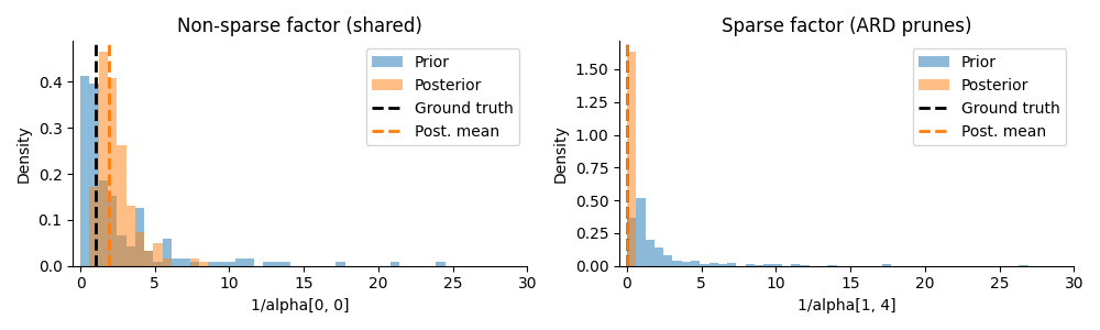
The sparse factor shows posterior concentration near zero, demonstrating that ARD has correctly identified this factor as irrelevant for group 1.

Aggregate metric: subspace error

For the full loading matrix, we use a normalized subspace error that is invariant to column ordering:

\[e_{\text{sub}} = \frac{\|(I - \hat{M}(\hat{M}^\top\hat{M})^{-1}\hat{M}^\top)M\|_F} {\|M\|_F}\]

where \(M\) is ground truth and \(\hat{M}\) is the estimate. A value of 0 means the estimate captures the full column space of the ground truth.

def subspace_error(M_true: np.ndarray, M_est: np.ndarray) -> float:
    """Compute normalized subspace error between ground truth and estimate."""
    # Projection onto null space of M_est
    # P_null = I - M_est @ pinv(M_est)
    M_est_pinv = np.linalg.pinv(M_est)
    P_null = np.eye(M_true.shape[0]) - M_est @ M_est_pinv

    # Projection of M_true onto null space
    residual = P_null @ M_true

    return np.linalg.norm(residual, "fro") / np.linalg.norm(M_true, "fro")

Compute subspace error for prior and posterior samples.

C_true = obs_params_true.C

e_sub_prior = np.array([subspace_error(C_true, s.C) for s in prior_samples])
e_sub_posterior = np.array([subspace_error(C_true, s.C) for s in posterior_samples])

# Also compute for the posterior mean
C_mean = model.obs_posterior.C.mean
e_sub_mean = subspace_error(C_true, C_mean)

# Shared bins for comparable histograms
bins = np.linspace(0, 1, 50)

fig, ax = plt.subplots(figsize=(6, 3))

ax.hist(e_sub_prior, bins=bins, alpha=0.5, label="Prior", color="C0", density=True)
ax.hist(
    e_sub_posterior, bins=bins, alpha=0.5, label="Posterior", color="C1", density=True
)
ax.axvline(e_sub_mean, color="C1", linestyle="--", linewidth=2, label="Post. mean")

ax.set_xlim(0, 1)
ax.set_xlabel("Subspace error $e_{sub}$")
ax.set_ylabel("Density")
ax.set_title("Loading matrix recovery: prior vs posterior")
ax.legend()
ax.spines["top"].set_visible(False)
ax.spines["right"].set_visible(False)

plt.tight_layout()
plt.show()

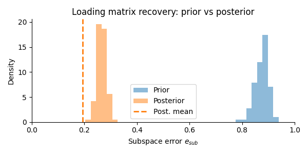
The posterior samples achieve much lower subspace error than prior samples, indicating that the learned distribution captures the ground truth column space.

print(f"Prior samples:     mean e_sub = {e_sub_prior.mean():.3f}")
print(f"Posterior samples: mean e_sub = {e_sub_posterior.mean():.3f}")
print(f"Posterior mean:    e_sub = {e_sub_mean:.3f}")

Prior samples:     mean e_sub = 0.875
Posterior samples: mean e_sub = 0.266
Posterior mean:    e_sub = 0.194