Simulating from the GFA model

This example walks through the Group Factor Analysis (GFA) generative model step-by-step, showing how hyperpriors, priors, and realizations work together to produce multi-group observations with shared and group-specific structure.

Imports

import matplotlib.pyplot as plt
import numpy as np

from latents.gfa.config import GFASimConfig
from latents.gfa.simulation import sample_observations, simulate
from latents.observation import (
    ObsParamsHyperPriorStructured,
    ObsParamsPrior,
    adjust_snr,
)
from latents.plotting import hinton_diagram
from latents.state import LatentsPriorStatic

Configure the simulation

We define the dataset dimensions and a sparsity pattern that determines which latent factors are present in which observation groups. This pattern creates shared factors (present in multiple groups) and group-specific factors (present in only one group).

n_samples = 100
y_dims = np.array([10, 10, 10])  # 3 groups, each with 10 observed dimensions
n_groups = len(y_dims)
x_dim = 7  # 7 latent factors

# Sparsity pattern: (n_groups x x_dim)
# - Finite values indicate a factor IS present in that group
# - np.inf indicates a factor is NOT present (will be pruned to zero)
#
# This pattern creates:
#   - Factor 0: shared across all groups
#   - Factors 1-3: shared between pairs of groups
#   - Factors 4-6: group-specific
sparsity_pattern = np.array(
    [
        [1, 1, 1, np.inf, 1, np.inf, np.inf],  # Group 0
        [1, 1, np.inf, 1, np.inf, 1, np.inf],  # Group 1
        [1, np.inf, 1, 1, np.inf, np.inf, 1],  # Group 2
    ],
)

Set up hyperpriors

The hyperprior controls how observation model parameters are sampled. ObsParamsHyperPriorStructured uses the sparsity pattern to set ARD (Automatic Relevance Determination) parameters.

The key parameters a_alpha and b_alpha control the Gamma prior on precision (inverse variance) of each loading column. Setting a_alpha=inf forces the corresponding precision to infinity, effectively zeroing out that factor for that group.

MAG = 100  # Controls variance of alpha; larger = tighter concentration
hyperprior = ObsParamsHyperPriorStructured(
    a_alpha=MAG * sparsity_pattern,
    b_alpha=MAG * np.ones_like(sparsity_pattern),
    a_phi=1.0,  # Observation noise shape
    b_phi=1.0,  # Observation noise rate
    beta_d=1.0,  # Mean offset precision
)

Sample observation parameters

The prior samples concrete parameter values (a “realization”) given the hyperprior. This produces loading matrices C, ARD precisions alpha, noise precisions phi, and mean offsets d.

rng = np.random.default_rng(seed=0)

prior = ObsParamsPrior(hyperprior=hyperprior)
obs_params = prior.sample(y_dims=y_dims, x_dim=x_dim, rng=rng)

print(f"Loading matrix C shape: {obs_params.C.shape}")
print(f"ARD precisions alpha shape: {obs_params.alpha.shape}")

Loading matrix C shape: (30, 7)
ARD precisions alpha shape: (3, 7)

Sample latent variables

The latent prior generates factor scores for each sample. For static (non-time-series) data, we use LatentsPriorStatic, which samples i.i.d. standard normal latents.

latents_prior = LatentsPriorStatic()
latents = latents_prior.sample(x_dim=x_dim, n_samples=n_samples, rng=rng)

print(f"Latents shape: {latents.data.shape}")  # (x_dim, n_samples)

Latents shape: (7, 100)

Generate observations

Given latents X and observation parameters, the generative model produces observations Y for each group:

\[\mathbf{y}^{(m)} = \mathbf{C}^{(m)} \mathbf{x} + \mathbf{d}^{(m)} + \boldsymbol{\epsilon}^{(m)}\]

where \(\boldsymbol{\epsilon}^{(m)} \sim \mathcal{N}(\mathbf{0}, \text{diag}(\boldsymbol{\phi}^{(m)})^{-1})\).

Y = sample_observations(latents, obs_params, rng=rng)

print(f"Observations Y shape: {Y.data.shape}")  # (sum(y_dims), n_samples)
print(f"Group dimensions: {Y.dims}")

Observations Y shape: (30, 100)
Group dimensions: [10 10 10]

All-in-one alternative

The steps above (hyperprior → prior → sample parameters → sample latents → sample observations) are wrapped in a single convenience function simulate():

sim_config = GFASimConfig(
    n_samples=n_samples,
    y_dims=y_dims,
    x_dim=x_dim,
    snr=1.0,
    random_seed=42,
)

sim_result = simulate(sim_config, hyperprior)
# sim_result contains: observations, obs_params, latents

Visualize ground truth

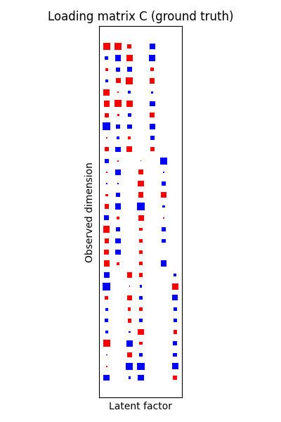
Hinton diagrams show the loading matrix structure. Square size indicates magnitude; color indicates sign (red = positive, blue = negative). The sparsity pattern is visible: columns with inf in the sparsity pattern have near-zero values for those groups.

# Stack loading matrices for all groups
C = obs_params.C  # (sum(y_dims), x_dim)

plt.figure(figsize=(4, 6))
hinton_diagram(C)
plt.title("Loading matrix C (ground truth)")
plt.xlabel("Latent factor")
plt.ylabel("Observed dimension")
plt.tight_layout()
plt.show()

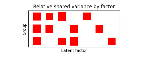
We can also visualize the ARD parameters, which control how much variance each factor explains in each group. Factors with inf in the sparsity pattern have very high precision (near-zero variance contribution).

alpha_inv = 1 / obs_params.alpha  # (n_groups, x_dim)
alpha_inv_rel = alpha_inv / np.sum(alpha_inv, axis=1, keepdims=True)

plt.figure(figsize=(5, 2))
hinton_diagram(alpha_inv_rel)
plt.title("Relative shared variance by factor")
plt.xlabel("Latent factor")
plt.ylabel("Group")
plt.tight_layout()
plt.show()

Effect of SNR

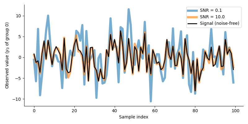
The signal-to-noise ratio (SNR) controls how much observation noise obscures the latent structure. Here we show the noise-free signal alongside noisy observations at different SNR levels.

# Compute noise-free signal for dimension 0 of group 0
# Signal = C @ X + d (no noise term)
y_signal = obs_params.C[0, :] @ latents.data + obs_params.d[0]  # (n_samples,)

samples = np.arange(n_samples)

plt.figure(figsize=(8, 4))

for snr, color in zip([0.1, 10.0], ["C0", "C1"], strict=True):
    obs_params_snr = adjust_snr(obs_params, snr)
    Y_noisy = sample_observations(latents, obs_params_snr, rng)
    y_obs = Y_noisy.data[0, :]  # dim 0 of group 0
    plt.plot(samples, y_obs, alpha=0.6, linewidth=5, label=f"SNR = {snr}", color=color)
plt.plot(samples, y_signal, "k-", linewidth=2, label="Signal (noise-free)")

plt.xlabel("Sample index")
plt.ylabel("Observed value ($y_0$ of group 0)")
plt.gca().spines["top"].set_visible(False)
plt.gca().spines["right"].set_visible(False)
plt.legend()
plt.tight_layout()
plt.show()