Fitting GFA to simulated data

This example demonstrates fitting a GFA model to synthetic data and validating parameter recovery against known ground truth.

Imports

import logging
import sys

import matplotlib.pyplot as plt
import numpy as np

import latents.gfa.analysis as gfa_analysis
from latents.callbacks import LoggingCallback
from latents.gfa import GFAFitConfig, GFAModel
from latents.gfa.config import GFASimConfig
from latents.gfa.simulation import simulate
from latents.observation import ObsParamsHyperPriorStructured
from latents.plotting import hinton_diagram

# Configure logging to stdout (sphinx-gallery captures stdout, not stderr)
# force=True ensures fresh config even if another example ran first
logging.basicConfig(
    level=logging.INFO, format="%(message)s", stream=sys.stdout, force=True
)

Simulate data

We generate synthetic data with known ground truth parameters so we can evaluate how well the model recovers the true latent structure. This setup is identical to Simulating from the GFA model.

n_samples = 100
y_dims = np.array([10, 10, 10])
x_dim = 7

# Sparsity pattern defining shared and group-specific factors
sparsity_pattern = np.array(
    [
        [1, 1, 1, np.inf, 1, np.inf, np.inf],
        [1, 1, np.inf, 1, np.inf, 1, np.inf],
        [1, np.inf, 1, 1, np.inf, np.inf, 1],
    ],
)

MAG = 100
hyperprior = ObsParamsHyperPriorStructured(
    a_alpha=MAG * sparsity_pattern,
    b_alpha=MAG * np.ones_like(sparsity_pattern),
    a_phi=1.0,
    b_phi=1.0,
    beta_d=1.0,
)

sim_config = GFASimConfig(
    n_samples=n_samples,
    y_dims=y_dims,
    x_dim=x_dim,
    snr=1.0,
    random_seed=0,
)

sim_result = simulate(sim_config, hyperprior)
Y = sim_result.observations
obs_params_true = sim_result.obs_params

Configure fitting

GFAFitConfig controls the fitting procedure. Key parameters:

• x_dim_init: Initial latent dimensionality. Set larger than expected; ARD will prune unnecessary dimensions.

• fit_tol: Convergence tolerance on relative ELBO change.

• prune_x: Whether to remove dimensions with negligible variance.

config = GFAFitConfig(
    x_dim_init=10,  # Larger than true x_dim=7; ARD will prune extras
    fit_tol=1e-8,
    max_iter=20000,
    random_seed=0,
    prune_x=True,
    prune_tol=1e-7,
)

Fit the model

fit() runs variational inference. Use LoggingCallback to log key milestones.

model = GFAModel(config=config)
model.fit(Y, callbacks=[LoggingCallback()])

fit.started [n_samples=100; y_dims=[10 10 10]; x_dim=10]
fit.x_dim_pruned [n_removed=1; x_dim_remaining=9; iteration=14]
fit.x_dim_pruned [n_removed=1; x_dim_remaining=8; iteration=17]
fit.x_dim_pruned [n_removed=1; x_dim_remaining=7; iteration=86]
fit.converged [iteration=2493]

GFAModel(fitted=True, config=GFAFitConfig(x_dim_init=10, fit_tol=1e-08, max_iter=20000, prune_x=True, prune_tol=1e-07, save_x=False, save_c_cov=False, save_fit_progress=True, random_seed=0, min_var_frac=0.001))

Check convergence

After fitting, inspect convergence diagnostics:

• model.flags: Status flags (converged, hit max iterations, etc.)

• model.tracker.plot_lb(): ELBO (evidence lower bound) over iterations

model.flags.display()

Converged: True
Decreasing lower bound: False
Private variance floor: False
Latent dimensions removed: 3

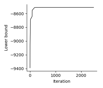
The ELBO should increase monotonically and plateau at convergence.

model.tracker.plot_lb()

Compare loading matrices

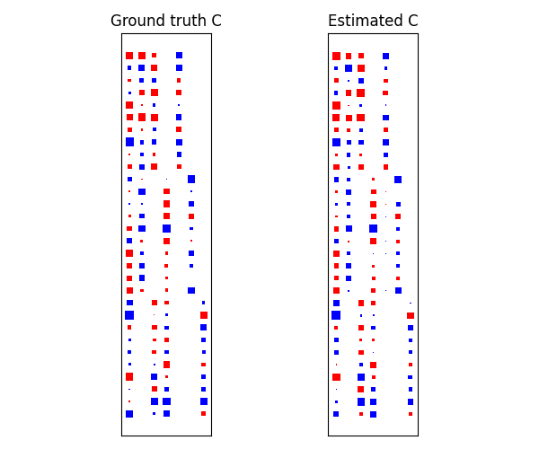
Factor models have inherent ambiguities: columns can be reordered and sign-flipped without changing the model. For ground truth comparison, we manually align columns.

# Manual alignment (determined by inspection)
reorder = np.array([1, 4, 3, 6, 0, 2, 5])
rescale = np.array([-1, -1, 1, 1, 1, 1, 1])

fig, axes = plt.subplots(1, 2, figsize=(6, 5))

axes[0].set_title("Ground truth C")
hinton_diagram(obs_params_true.C, ax=axes[0])

axes[1].set_title("Estimated C")
C_est_aligned = model.obs_posterior.C.mean[:, reorder] * rescale
hinton_diagram(C_est_aligned, ax=axes[1])

plt.tight_layout()
plt.show()

ARD and dimensionality discovery

ARD (Automatic Relevance Determination) prunes unnecessary latent dimensions by driving their precision to infinity. We visualize the relative shared variance explained by each factor.

alpha_inv_true = 1 / obs_params_true.alpha
alpha_inv_rel_true = alpha_inv_true / np.sum(alpha_inv_true, axis=1, keepdims=True)

alpha_inv_est = 1 / model.obs_posterior.alpha.mean
alpha_inv_rel_est = alpha_inv_est / np.sum(alpha_inv_est, axis=1, keepdims=True)

fig, axes = plt.subplots(2, 1, figsize=(5, 3))

axes[0].set_title("Ground truth ARD")
hinton_diagram(alpha_inv_rel_true, ax=axes[0])

axes[1].set_title("Estimated ARD (reordered)")
hinton_diagram(alpha_inv_rel_est[:, reorder], ax=axes[1])

plt.tight_layout()
plt.show()

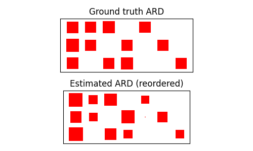
Notice that the model started with 10 latent dimensions but ARD identified only 7 as meaningful, matching the true dimensionality.

print(f"Initial dimensions: {config.x_dim_init}")
print(f"Final dimensions:   {model.obs_posterior.x_dim}")
print(f"True dimensions:    {x_dim}")

Initial dimensions: 10
Final dimensions:   7
True dimensions:    7

We can also inspect the discovered sparsity pattern — which factors are significant in each group. This uses compute_dimensionalities(), which thresholds the relative shared variance explained by each factor. Again, we manually align the columns with the ground truth for comparison.

_, sig_dims, _, _ = model.obs_posterior.compute_dimensionalities()
print(sig_dims[:, reorder].astype(int))

[[1 1 1 0 1 0 0]
 [1 1 0 1 0 1 0]
 [1 0 1 1 0 0 1]]

Predictive performance

We evaluate the model using leave-group-out prediction: for each group, predict its observations from the other groups via the shared latents.

R2, MSE = gfa_analysis.predictive_performance(Y, model.obs_posterior)
print(f"Leave-group-out R²:  {R2:.4f}")
print(f"Leave-group-out MSE: {MSE:.4f}")

Leave-group-out R²:  0.3545
Leave-group-out MSE: 5.1290