GFA dimensionality recovery benchmarks

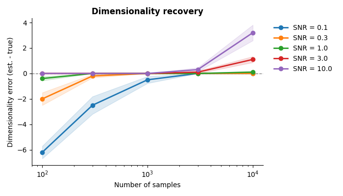
These benchmarks evaluate how well post-hoc dimensionality selection recovers the true number of latent dimensions across varying sample sizes and noise levels.

The model is fit with more latent dimensions than the true data-generating process (x_dim_init = 20, x_dim_true = 10), and dimensionality is determined after fitting via compute_dimensionalities() using default cutoffs (cutoff_shared_var = 0.02, cutoff_snr = 0.001).

Fixed parameters:

• x_dim_true = 10, x_dim_init = 20

• n_groups = 1, y_dim_per_group = 50

• 10 runs per grid point

The metric is signed dimensionality error: x_dim_effective - x_dim_true. Positive values indicate overestimation.

Imports and setup

from pathlib import Path

import matplotlib.pyplot as plt
import pandas as pd

from benchmarks.plotting import plot_dimensionality

# Path to pre-computed benchmark data
DATA_DIR = Path("../data")
GFA_DIM_DIR = DATA_DIR / "gfa/dimensionality"

Dimensionality recovery across samples and SNR

The horizontal dashed line at 0 marks perfect recovery. Two distinct regimes emerge:

Low SNR, few samples (negative errors): The model underestimates dimensionality — true latent dimensions cannot be distinguished from noise. From a Bayesian perspective, this reflects principled conservatism: with weak evidence, the posterior favors simpler models. More data resolves this, and errors approach zero.

High SNR, many samples (positive errors): The model overestimates dimensionality — extra dimensions survive the post-hoc significance cutoff. With abundant data and low noise, the cost of overfitting is small, and the model assigns non-negligible variance to spurious dimensions.

This behavior is not specific to GFA or to ARD-based selection; it has been reported for simpler methods like factor analysis with cross-validation (Williamson et al., 2016), and for Bayesian time series methods like mDLAG (Gokcen et al., 2025).

The sweet spot lies between these extremes — enough data to identify the true structure, but not so much statistical power that spurious dimensions become indistinguishable from real ones. In practice, users should treat the default cutoffs as a starting point and consider validating dimensionality estimates against held-out data or domain knowledge, particularly in data-rich regimes.

df = pd.read_csv(GFA_DIM_DIR / "n_samples_snr.csv")
plot_dimensionality(df)
plt.show()