GFA runtime benchmarks

These benchmarks validate theoretical computational complexity and help users anticipate fitting times for their datasets.

Each sweep varies one factor while holding others at sensible defaults:

• n_samples = 1000, y_dim = 100/group, x_dim = 3, n_groups = 2

Results show mean ± SEM across 10 independent runs per configuration.

Imports and setup

from pathlib import Path

import matplotlib.pyplot as plt
import pandas as pd

from benchmarks.plotting import display_system_info, plot_runtime_sweep

# Paths to pre-computed benchmark data
DATA_DIR = Path("../data")
GFA_RUNTIME_DIR = DATA_DIR / "gfa/runtime"


def load_runtime_sweep(name: str) -> pd.DataFrame:
    """Load a runtime sweep CSV."""
    return pd.read_csv(GFA_RUNTIME_DIR / f"{name}.csv")

Scaling with number of samples

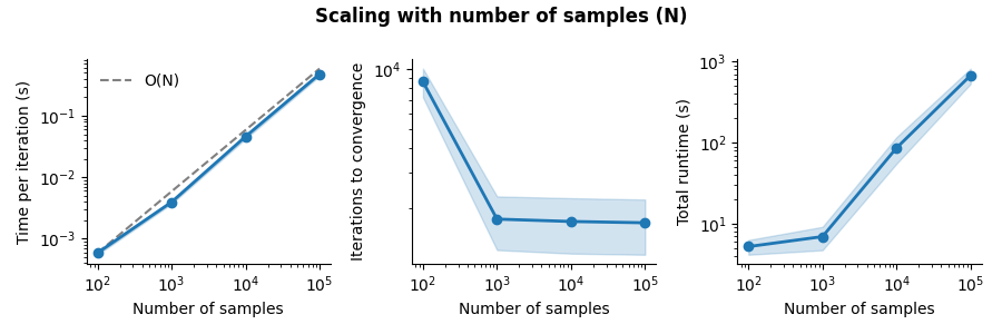
Theoretical scaling: O(N) — linear in number of samples.

The latent states are inferred by iterating over samples, and the updates for all other parameters are independent of sample count. Total complexity is dominated by the O(N) latent inference operations.

df_n_samples = load_runtime_sweep("n_samples")
plot_runtime_sweep(
    df_n_samples,
    title="Scaling with number of samples (N)",
    xlabel="Number of samples",
    ref_slope=1,
    ref_label="O(N)",
)
plt.show()

Scaling with observed dimensionality

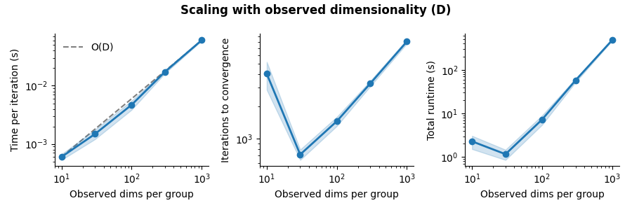
Theoretical scaling: O(D) — linear in total observed dimensions.

Per-group computations scale linearly with that group’s dimensionality. With fixed latent dimensionality, the dominant cost is matrix-vector operations that scale as O(D).

df_y_dim = load_runtime_sweep("y_dim_per_group")
plot_runtime_sweep(
    df_y_dim,
    title="Scaling with observed dimensionality (D)",
    xlabel="Observed dims per group",
    ref_slope=1,
    ref_label="O(D)",
)
plt.show()

Scaling with latent dimensionality

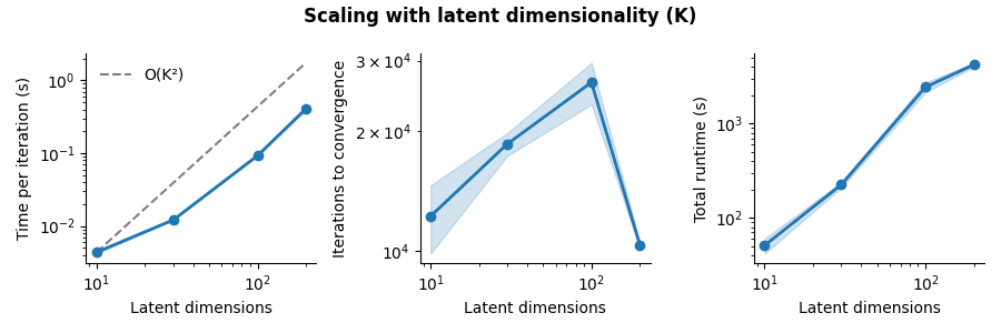
Theoretical scaling: O(K³) — two steps involve K x K matrix inversions: latent inference (one K x K inverse) and loading inference (D separate K x K inverses).

Empirical scaling: O(K²) up to K = 200. At these matrix sizes, well within typical use, optimized LAPACK routines run faster than the asymptotic cubic cost would predict.

df_x_dim = load_runtime_sweep("x_dim")
plot_runtime_sweep(
    df_x_dim,
    title="Scaling with latent dimensionality (K)",
    xlabel="Latent dimensions",
    ref_slope=2,
    ref_label="O(K²)",
)
plt.show()

Scaling with number of groups

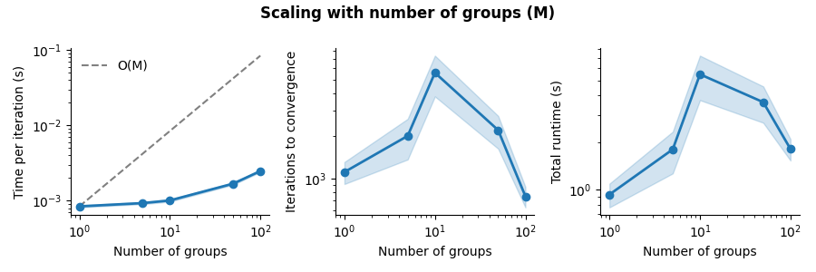
Theoretical scaling: ~O(1) with total observed dimensionality fixed.

This sweep holds total D = 100 constant while varying the number of groups. Per-group dimensions decrease as group count increases, so the dominant per-iteration cost (proportional to total D) stays constant. The mild increase in cost reflects per-group bookkeeping. The O(M) reference line is shown for comparison; actual growth is sublinear.

df_n_groups = load_runtime_sweep("n_groups")
plot_runtime_sweep(
    df_n_groups,
    title="Scaling with number of groups (M)",
    xlabel="Number of groups",
    ref_slope=1,
    ref_label="O(M)",
)
plt.show()

Benchmark environment

System information for reproducibility. Runtime benchmarks are sensitive to hardware and software versions.

display_system_info(DATA_DIR / "system_info.json")

Hardware
--------
CPU: AMD Ryzen 9 6900HX with Radeon Graphics
Cores: 8 physical, 16 logical
RAM: 60.6 GB

Software
--------
Python: 3.11.14
NumPy: 2.3.5
SciPy: 1.16.3
Latents: 0.0.5

Operating System
----------------
System: Linux
Distribution: Pop!_OS 22.04 LTS
Kernel: 6.17.9-76061709-generic